Why is this a cat?

In other words, “How do you recognize this cat?” Actually, I’m not so interested in how you see, but rather how computers see, because they’ve gotten a lot better at seeing and we don’t fully understand how they do it. For those coming to this blog who don’t know, Convolutional Neural Networks (ConvNets) are the models that have allowed computers to do reasonably well at a wide variety of visual tasks. There are some intuitions about how ConvNets work, but it can be hard to find examples of them. This is the first of two posts. In this first part I’ll tell you about Convolutional Neural Networks, some work others have done to gain intuition about them, and some opportunities these approaches miss. The next post will introduce a new visualization technique to help gain more intuition.

(You can see part 2 of this blog here.)

(Convolutional) Neural Networks – Building Layers of Patterns

Others have done quite a good job of introducing Neural Networks (NNs) and ConvNets, so I won’t spend much time on that. You can find a variety of pointers in the footnote at the end of this sentence¹. I’ll still try to introduce the important concepts for this blog as I go along.

Though they’ve been around since the ’80s, ConvNets became really popular after faster computers and more data allowed them to win the ImageNet Large Scale Visual Recognition Challenge in 2012². Since then, this type of model has been raised from obscurity to become a fundamental part of Computer Vision. We’ve discovered they’re pretty good at a lot more than telling you an image contains a cat.

ConvNets work by transforming an input (the cat image) in multiple steps or layers. The first layer, the input, corresponds to image pixels and the last layer, the output, has one number for each object class the image might contain (the 1000 classes from the ILSVRC 2012 challenge). Each layer looks for patterns in its input, transforming them into new outputs where higher layers look for more complex patterns until the final layer produces outputs that correspond to whatever you’re interested in (i.e., it labels the image a cat).

A useful way to think of a neural network is in terms of the nodes – called units or neurons – which look for or try to detect patterns. Below is a network with 4 layers, each containing some nodes (though the input nodes aren’t shown). On the left is the input with 5 nodes and on the right is the output with 1 node. The first hidden (middle) layer contains 3 nodes and the 2nd has 4.

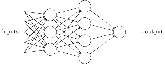A simple Neural Network with 4 layers (including input and output)³.

In normal neural networks each unit corresponds to a single number, but in ConvNets they correspond to images. The network we’ll be using (AlexNet) has 9 layers (0 through 8) and each layer has hundreds of neurons. This scale (many layers, many neurons) is important for understanding images well.

The important idea for this article is the connections between units. Each unit is connected to all the units in the previous layer so it can search for patterns in those units and become highly active when it sees the patterns it’s looking for. Since there are multiple layers, deeper (toward the output) units are looking at patterns of patterns of patterns…. so each unit depends on the ones that came before it in a hierarchical fashion. The hierarchies of neurons allow efficient representation of complex patterns in terms of simpler patterns.

Something we Don’t Know

Crucially, the patterns in these systems are learned from examples, and this is where our understanding of the system starts to fail. To train a ConvNet, we show it hundreds of thousands of cats, dogs, boats, birds, etc., and adjust the patterns seen by neurons at all layers so that the last layer says cat when the image contains a cat and not otherwise⁴. This ability to get a working system from only a vague specification makes the model possible – humans couldn’t manually specify all the patterns – but it also means we sacrifice some understanding. In one sense I understand exactly how the ConvNets work because I can implement them in code and they make good predictions once trained. In another sense I have no idea how the things work because I don’t know what patterns they’re looking for.

An interesting thing about ConvNets is that it even has small bits which we might be able to intuit. Consider Deep Blue, IBM’s program which famously beat the reigning world champion at chess. At some point a team of programmers coded the thing up, so they clearly know how Deep Blue works. However, a similar problem to the ConvNets problem appears. If you ask one of the programmers to tell you why the machine made a particular move she can’t tell you in a way that fits into the understanding of even the most seasoned chess player.

There aren’t any patterns to understand. When asked to make a move, Deep Blue searches through all possible future moves and has some rules to help it pick the best. By itself this would be impossible, but there are a few nice algorithmic tricks and well chosen rules that allowed it to perform as well as it did. However, those tricks fit into a human understanding of how to play chess in the same way the brute force method fits into such an understanding: they don’t.

On the other hand, humans can describe, and even teach how they play chess. It’s harder to describe how we see.

Why is this a cat?

Here’s my answer:

The thing in the center has eyes, a flat, pink nose, and a small mouth. It also has pointy ears which compose with the previous features to form a head with ears on top and mouth on the bottom. Furthermore, it has whiskers, and is quite furry. Its expression is amusing, but has little to do with it being a cat.

That’s a start, but it isn’t precise enough. I can’t use it to write an algorithm that sees because the description isn’t in terms of any useful input. I don’t (nor do computers) have a furry sense, an ear sense, or a mouth sense – that’s what vision gives me – yet I described what I see in terms of those fundamental components. It would be useful if I could recursively describe each of these parts in further detail until each complex visual pattern is detailed in terms of the input.

Evidence suggests this is at least very hard. Computer Vision is the name of the field which has been trying to do it for decades. Come up with a candidate description, test it by implementing it on a computer, fail, repeat⁵.

However, ConvNets seem to be able to do it, so let’s try to understand them.

Visualizing Individual Units

Especially since the ILSVRC challenge in 2012, many methods have been proposed to understand the patterns learned by ConvNets. The kind of understanding I’m interested in is an intuitive understanding of why a ConvNet makes a particular choice. It’s hard to describe how we see in words, so it might seem even more futile for ConvNets. However, our precise computational understanding of ConvNets allows us to generate images with certain specific meanings. Fortunately, our visual system can often understand these visualizations and thereby understand something about ConvNets.

The next part gets researchy, so you can skip it if you get lost. All you need to know is that we can generate images that highlight the pixels a particular neuron cares about so that changing those pixels in the original image would greatly effect the neuron’s activation, but changing other pixels wouldn’t have such a great effect. That’s how these visualizations relate neurons to pixel space. Make sure you visit the examples section to get an idea of what the visualizations mean, because that’s the next step.

Ways to Visualize ConvNets

So far we have two ways to generate visualizations:

1. Optimization in Image Space (uses gradients)

   Training a ConvNet is just adjusting the patterns (free variables) that neurons look for in images (fixed variables) so the neurons become more and more likely to associate the patterns of a cat image with the label “cat.” Instead, this visualization method leaves patterns (fixed variables) alone and adjusts images (free variables) so the neurons are more and more likely to see the patterns they want to call “cat”. Note that these methods start with a blank image and optimize from there instead of starting with a real image and perturbing it, so these techniques are not image specific. They simply ask “What image would the ConvNet like to see?”

   Simonyan, Vedaldi, and Zisserman have done some nice work with this method, as have Mahendran and Vedaldi. Some earlier work was done by Erhan et. al. Here’s a visualization which was generated to maximize the flamingo recognizing neuron using this method. You can clearly see “flamingo elements.” I wouldn’t call the thing a flamingo, but our ConvNet would.

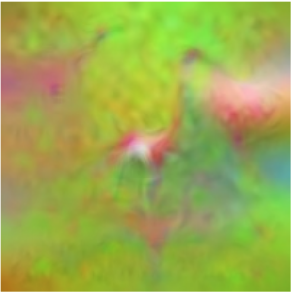   From figure 8 of [Mahendran and Vedaldi].

2. Gradients (just gradients, sort of)

   Another technique tries to show how changing certain pixels will change a desired neuron (again, e.g., a neuron trained to recognize cats). That is, it just visualizes the gradient of a particular neuron with respect to the image. This technique is image specific. It asks “Which pixels in this one particular picture made the cat activation high?”

   Actually, I lied. Visualizing the pure gradients is not very satisfying, as shown in Simonyan, Vedaldi, and Zisserman paper. Zeiler and Fergus created a “deconv” visualization which is mathematically similar to the gradient image, except it uses a slightly different function to compute the backward pass of the ReLU, so it can’t be called a gradient (explained in Simonyan, Vedaldi, and Zisserman and quite clearly in the guided backprop paper).

   Deconv visualizations by Zeiler and Fergus were the first to figure out this method. A more recent extension by Springenberg, Dosovitskiy, Brox, and Riedmiller is called guided bakprop. It refines the idea and makes it work for fully connected layers (at least those in AlexNet) by adding another restriction to the backward pass of the ReLU unit (again, their paper has an excellent explanation). In contrast to the first type of visualization, these methods focus on intermediate layers and individual neurons rather than output layers and the ConvNet as a whole.

Note that the second method allows questions about specific images and specific neurons, which is good since I want to find out how a specific cat is recognized. Because it works for fully connected layers and I find the visualizations crisper, we’ll use guided backprop. There are some other cool techniques you can read about in the footnote at the end of this sentence⁶.

Examples

Now let’s use guided backprop to visualize a couple neurons in different layers. Here are visualizations of neurons 4 and 65 from layer conv1 (after the ReLU, but not after pooling):

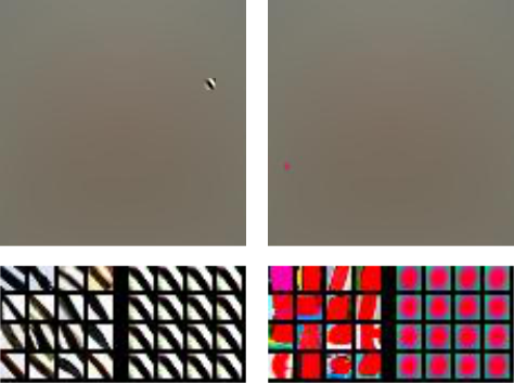
conv1_4 and conv1_65

The top of each side contains one of the “gradient” images the method produces, which means that changing the non-gray pixels in the original image will likely raise the activation of the corresponding neuron (conv1_4 or conv_65). It’s sometimes hard to determine exactly what semantic feature of the highlighted pixels the ConvNet responds to, so the bottom images help with that. These show two grids of patches which are chosen from 1000s of potential images instead just Grumpy Cat. The right sides of these images show “gradient” patches which highly activate the same neuron (black diagonals and red blobs). The left sides show the corresponding patches cropped from the original images. As some readers probably already know, conv1 learns to look for simple features which are easy to relate to pixels – e.g., oriented edges and colored blobs.

If you’re familiar with the type 2 visualizations from the previous section then you might wonder why these visualizations are much larger and mostly gray. Typically the non-gray section is cropped out of the gray because the gray sections have 0 gradient and are uninformative, as in the bottom part of the visualization. To be consistent with future visualizations I left the whole image intact, which means it’s mostly gray and insignificant, but location information is preserved.

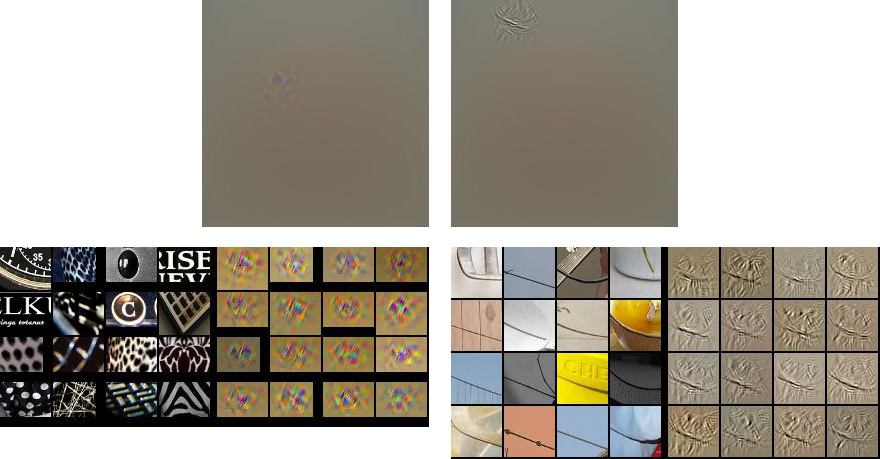
conv2_174 and conv2_69

conv2 is a bit less straightforward to understand than conv1. It’s hard to say what the neuron on the left seems to be looking for. Perhaps it’s a black or white background with some sort of clutter from the other color. I don’t see inuitively how such a pattern could contribute to recognition of ILSVRC object classes because I can’t imagine it (whatever it is) appearing very often. It’s also hard to find a rule that directly relates it to image pixels, but none of this necessarily means the neuron is useless. Unit 69 is clearly looking for mostly horizontal lines that go up slightly to the left. It’s nice that the unit is invariant to context (shower tiles, arm band, bowl) and I recognize that this sort of line might appear in a variety of objects. Still, I’m not sure how the fuzzy bits around the line in the gradient images relate to pixels. The visualization is hard to connect to either input or output.

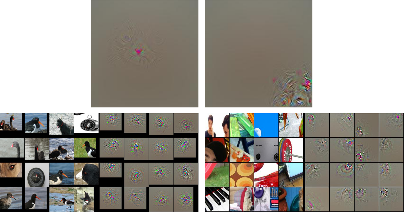
conv5_137 and conv4_269

Deeper layers capture more abstract concepts like the beak of a bird (conv5_137), which also activates highly in response to Grumpy Cat’s nose. Certain features like conv4_269 respond to specific patterns which are clearly at a larger scale than conv1 or conv2, but it’s hard to identify exactly how they might be useful. It’s hard to come up with a rule to extract either pattern from pixels.

What the Visualizations Don’t Say

In each example it was easy to understand the neurons in input/pixel space (e.g., conv1_4 is an edge filter), easy to understand the neurons in output space (e.g., conv5_137 should probably fire for birds), or it was hard to understand the neurons in either space (e.g., conv2_174). These visualizations are nice, but the inability to understand any neuron in terms of both input and output prevents us from understanding how ConvNets see and how they connect input to output. To be more specific,

1. These visualizations can sometimes confirm (qualitatively) that particular neurons select for concepts humans can label or for concepts that humans can connect directly to pixel space ⁷.

2. The first interpretation is limited to certain high level neurons. We can see that middle layers of neurons might be useful, but we don’t really know why. They need to be related in specific ways to either the gabor filters (oriented edge detectors) or the high level object parts, but we can’t intuit those ways.

3. Even though we can relate some things in specific ways (e.g., a head should have an ear), we don’t know for sure that the ConvNet is doing that (though it’s a pretty reasonable guess :). However, it could also be relating unknown parts in strange or (if you want to go that far) unwanted ways. These visualizations don’t say that the head is made up of pointy ears, a pink nose, whiskers, etc. We might know what things make up a head, but what is conv2_174 a part of?

These missing relationships are a fundamental part of ConvNets. They learn hierarchies of features. Of course hierarchies are graphs that have both nodes and edges, so to understand hierarchies we need to talk about the edges⁸.

Conclusion

In this post I started to explore how we understand ConvNets through visualization. Current techniques focus on individual neurons and allow us to analyze patterns a ConvNet recognizes, but they don’t show how those patterns relate to one another. The latter part is essential because ConvNets are supposed to work by composing more complex patterns out of simpler ones. I’ll try to investigate the edges in my next post.

Update: Check out part 2 of this blog here.

Acknowledgements

Thanks to Dan Cogswell and Dhruv Batra for their comments and suggestions.

---