Visualizing Feature Composition
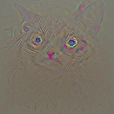
My last post described Convolutional Neural Networks (ConvNets) and some obstacles to understanding them. ConvNets identify objects in images by computing layers of features and using the last layer for object identification rather than directly using the input. Layers closer to the input capture low level visual concepts (e.g., edges and colors) and deeper layers capture higher level concepts (e.g., faces). We visualized features with “gradient” images (like the one above) which highlighted image pixels that had a significant effect on the feature in question. The conclusion was that ConvNets compute features that detect eyes and noses, but there wasn’t much intuition about how those eyes and noses are computed.
Here I’ll introduce a visualization technique that tries to do that. Instead of visualizing individual neurons, we’ll look at how neurons are related. A nose detector is made from a combination of features in the previous layer. To understand such a composition of features we’ll relate visualizations from one layer to visualizations of adjacent layers.
All of the code I used to produce these visualizations is available on github!
What’s Missing from the Visualizations?
So far we’ve understood feature visualizations by explaining that they select for either (1) concepts humans can label at a high level (e.g., face) or (2) concepts that humans relate to pixels (e.g., edge; low level). The first occurs in deeper layers which are closer to the output and the second occurs in shallow layers which are close the input. We can see that middle layers of neurons might be useful because they capture structure—certain configurations of near-by pixels that occur more than others. But we do not have more specific intuition as for the very shallow and very deep features. This means we can’t fit the outputs (high level) and inputs (low level) of a ConvNet together intuitively. Even though we can relate some features in specific ways (e.g., a head should have an ear), these examples stay within the realm of low level or high level and do not cross boundaries. This problem is ill defined and purely one of intuition, so it’s not clear what a solution looks like, but it motivates the search for new visualization meethods.
ConvNets learn hierarchies of features. Hierarchies are graphs with nodes and edges, so to understand hierarchies we need to understand edges as well as nodes. It makes sense to visualize relationships between features.
One interesting visualization which already does this is DrawNet, from Antonio Torralba at MIT. This is a really neat visualization, which you should go check out (though perhaps later ;). It uses the empirical receptive fields from this paper about emerging object detectors along with a visualization that connects individual neurons that depend heavily on each other1. However, it’s still not image specific, so it can only say how a ConvNet would “like” to relate some parts to others instead of how a ConvNet does relate some parts to others.
One way to Visualize the Edges
Our strategy will be to show single-feature visualizations from different layers and connect them when one feature heavily influences another. You can skip to the examples if you want to avoid a small bit of math.
Edges
It would be nice to connect neurons in adjacent layers so they are only connected when
- both neurons detect a pattern in the input and
- the ConvNet says one neuron is heavily dependent on the other.
If the first doesn’t hold then we’ll end up visualizing a pattern which isn’t relative to the example at hand. If the second doesn’t hold then we’ll relate two features which the ConvNet does not think are related.
There’s a fairly natural way to do this. Consider some fully connected layer fc7
which produces activations \(h^7 \in \mathbb{R}^{d_7}\) using
Where \(h^6 \in \mathbb{R}^{d_6}\) is the output of the previous layer and
\(W^{6-7} \in \mathbb{R}^{d_7 \times d_6}\) is the weight matrix for layer fc7.
The following vector weights fc6 features highly if they are related to
feature \(i\) in fc7, satisfying (2):
The activation vector \(h_6\) directly represents patterns detected in fc6, satisfying (1).
That means an element-wise product of the two vectors scores
features highly when they satisfy both (1) and (2), and lower otherwise:
To relate a feature in layer 7 to layer 6 we can use the top 5 indices of this
vector to select the fc6 features to visualize. Because the
visualizations of fully-connected layers turns out to not be very informative and
because convolutional layers contribute the most to depth, we
need to be able to do this for the feature maps produced by convolutional layers.
Fortunately, the extension is simple and I’ll show it using
conv5 instead of fc7 and conv4 instead of fc6.
Instead of computing the gradient \(\partial h^7_i / \partial h^6\) we’ll define a function \(f\) and compute the gradient with respect to that function. Specifically, let \(f: \text{feature map} \rightarrow \mathbb{R}\) be the sum of all pixels in an image. Then we’ll compute
\[\partial f(h^5_i) / \partial h^4\]where \(h^5_i\) is a vector of all the pixels in the \(i\)th feature map
in conv5 and \(h^4\) is a vector of all the pixels in all chanels of conv4.
Then we can weight conv4 pixels using
This is a generalization of the first approach, where there is only 1 pixel to be summed up, so \(f\) becomes the identity function. That means it also extends to cases where a convolutional layer is connected to a fully-connect layer. For details, see the code here.
Here’s an example which shows the 600th fc6 neuron in terms of the
5 conv5 units (20, 154, 247, 159, and 222) which most contribute to it.
Hovering your mouse over the image causes it to zoom.
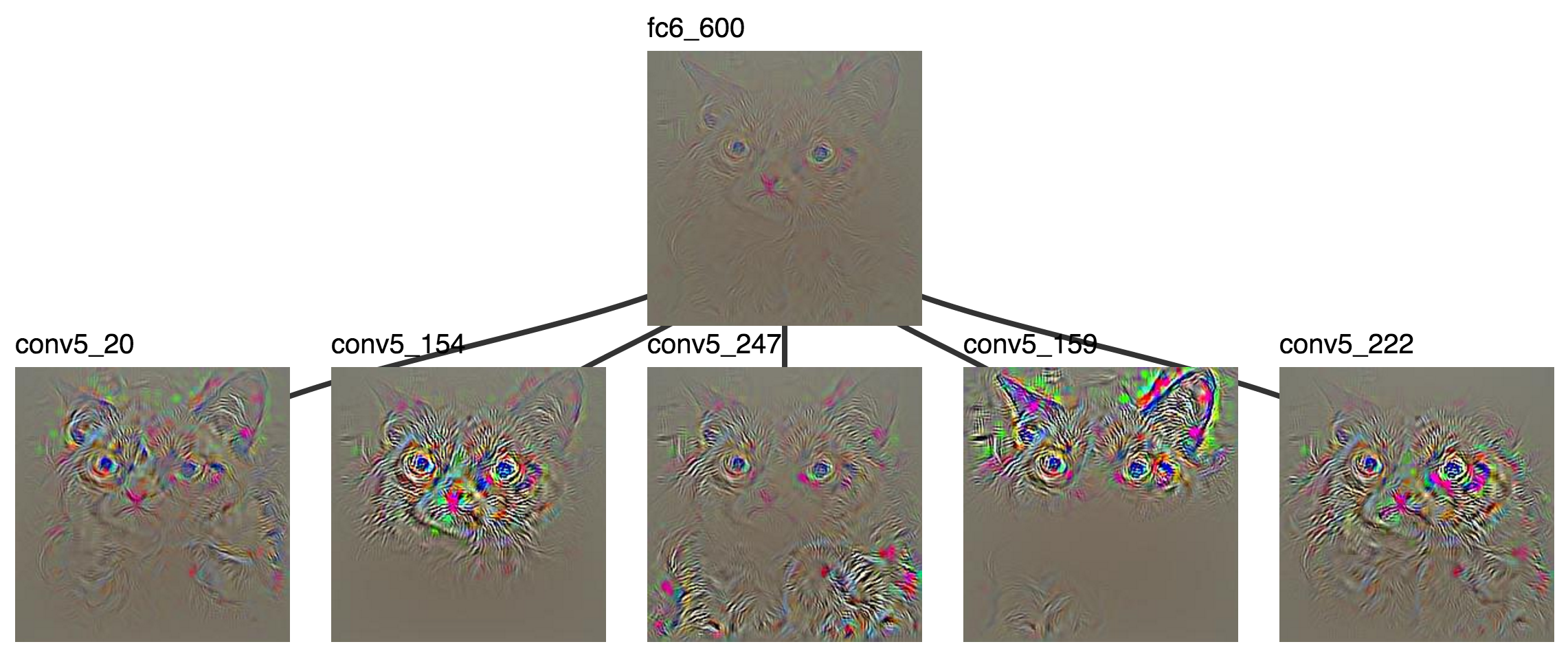
conv5 units which most contributed to the 600th fc6 activation
Local Visualization Paths
Before showing off some more examples, I have to mention one
trick I found helpful for creating relevant visualizations.
Visualizations of type 2 applied to convolutional
layers usually set all pixels but one (the highest activation)
to 0. When visualizing a unit in a convolutional
layer, say unit 44 in conv4, with respect to the layer above, unit 55 in conv5,
I could visualize unit 44 by taking a spatial max and setting all other
pixels to 0, however, that max pixel might be in a location far away from the
max pixel in unit 55, so those parts of the image might not be related and I might not be able to compare the two neurons.
To fix this I compute the gradient of unit 55 w.r.t. all units in conv4 then
set all conv4 feature maps to 0 except unit 44. This means a local region of pixels
is visualized in unit 44 instead of a single pixel, but that local region is guaranteed
to be centered around the highly activated pixel in unit 55, so I can relate the two units2.
Some Features in a Hierarchy
Why is this a cat?

Well… the highest fc8 activation is unit 284, which means “Siamese cat”.
Grumpy Cat turns out to be a Snowshoe Siamese according
to Wikipedia and the ILSVRC doesn’t have “Snowshoe Siamese”. Let’s start at fc8_284.
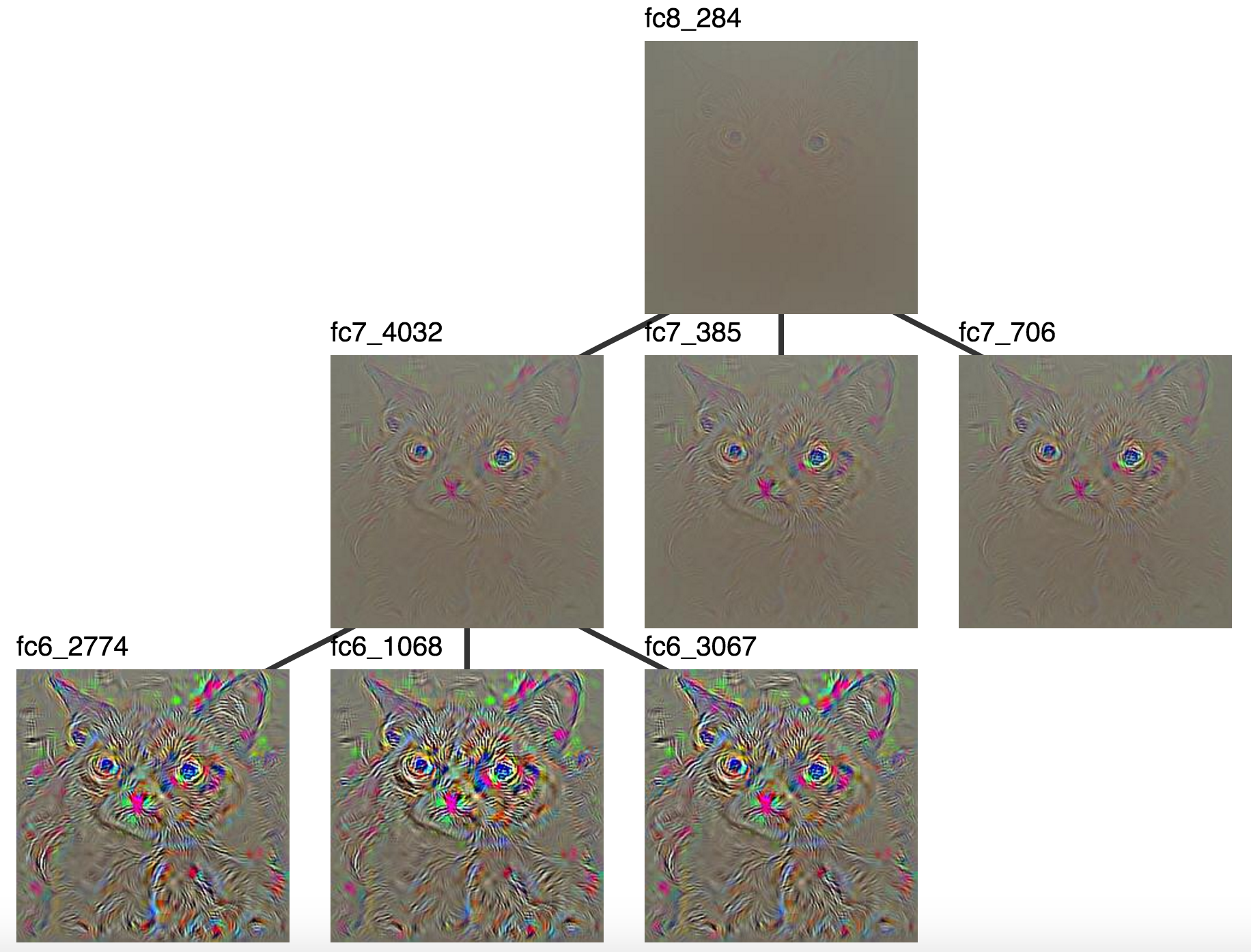
The “Siamese cat” neuron (fc8_284) along with units that highly activated it in fc7
and units that highly activated fc7_4032 in fc6.
Unfortunately, these don’t seem very interpretable, probably because these
layers have no spatial resolution. That means we can’t really relate classes
to pixels. However, the convolutional layers tell a different story. conv5
starts with high level interpretable features which we understand as cat
parts, so maybe we’ll be able to almost relate ConvNet outputs to inputs.
The conv5 visualizations rooted in fc8 were
quite saturated, so let’s start with a visualization rooted at fc6_1068.
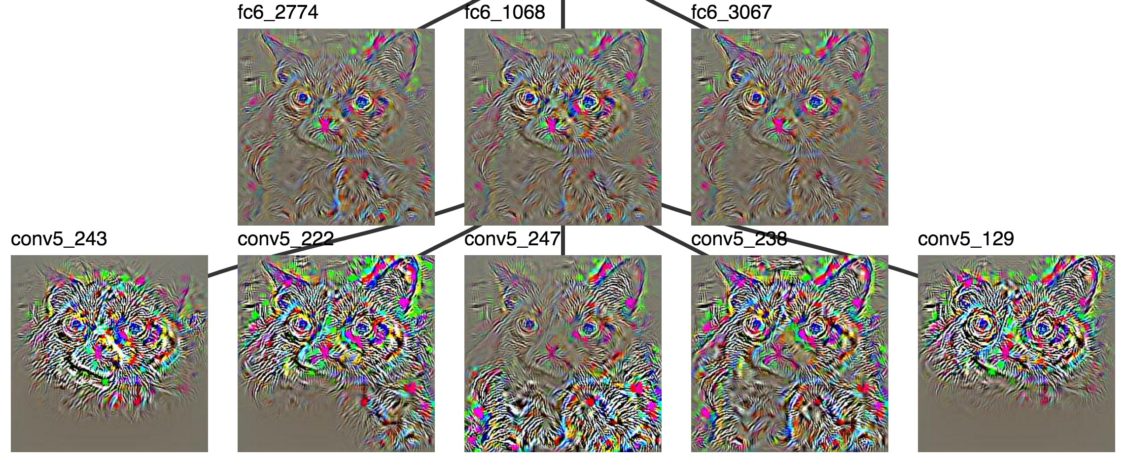
A highly activated fc6 unit and the conv5 units which most contributed to it.
Some units in conv5 are looking for faces. Some units are looking
for ears. The visualized units of conv5 which contribute to fc6_1068
seem to look for different parts of the cat which happen to show up in
different locations.
It becomes easier to tell what’s going on once the patch visualizations are added, but it’s hard to fit all 5 on the same screen, so let’s set aside two of them. These are looking for wheels (they look like eyes) and generic animal faces (lots and lots of conv5 activations look for some sort of animal face).
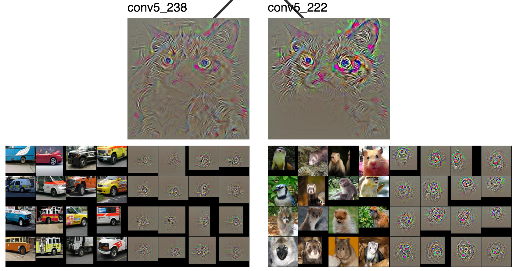
conv5_238 and conv5_222
Now we can focus on more interesting neurons.
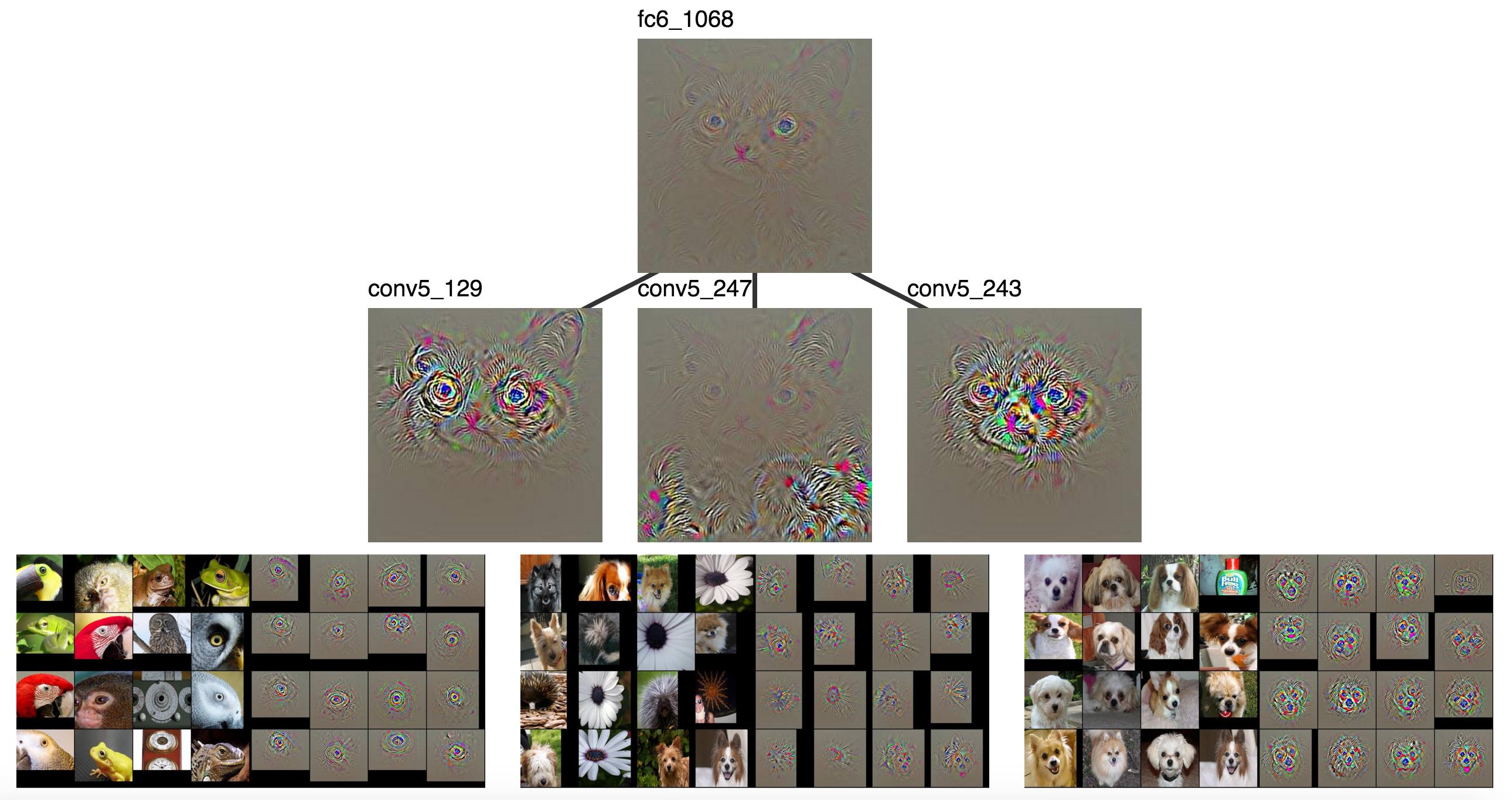
As shown previously, conv5_129, conv5_247, and conv5_243.
Clearly conv5_129 is looking for eyes, conv5_247 seems to be looking
at furry stuff, and conv5_243 is looking for dog faces.
Those are high level categories that could clearly contribute
to classifying Grumpy Cat as a cat.
furr + face + eye (perhaps tire) + … = cat
Let’s continue to conv4 to see what makes up a dog face.
Again, we’ll discard two neurons
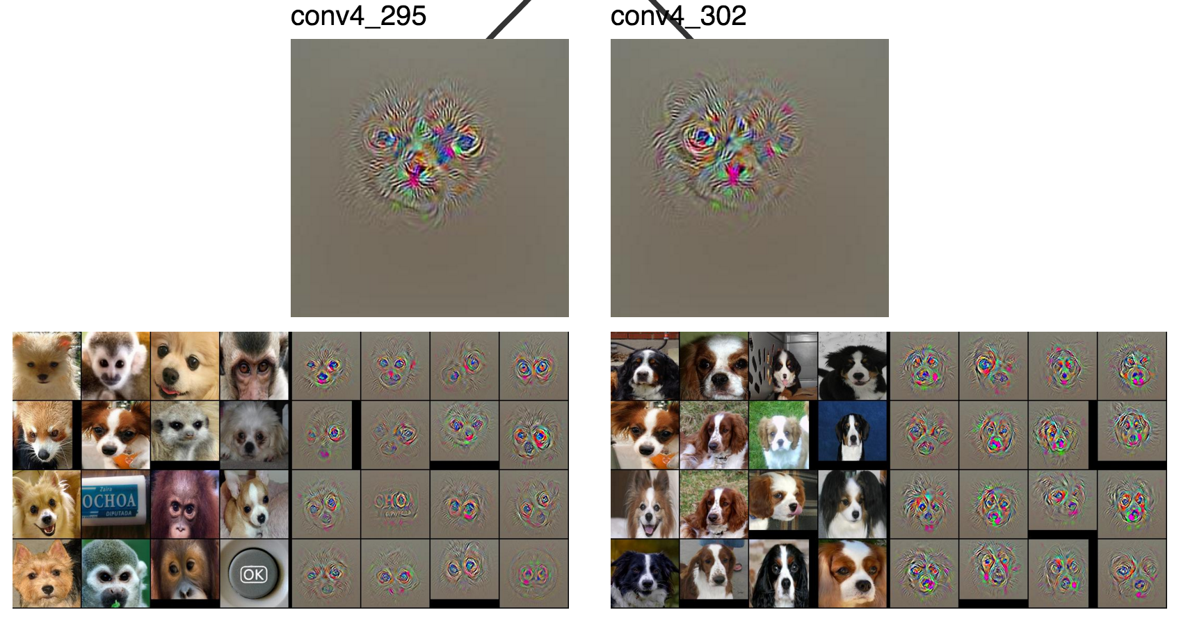
conv4_295 and conv4_302
and keep the rest.
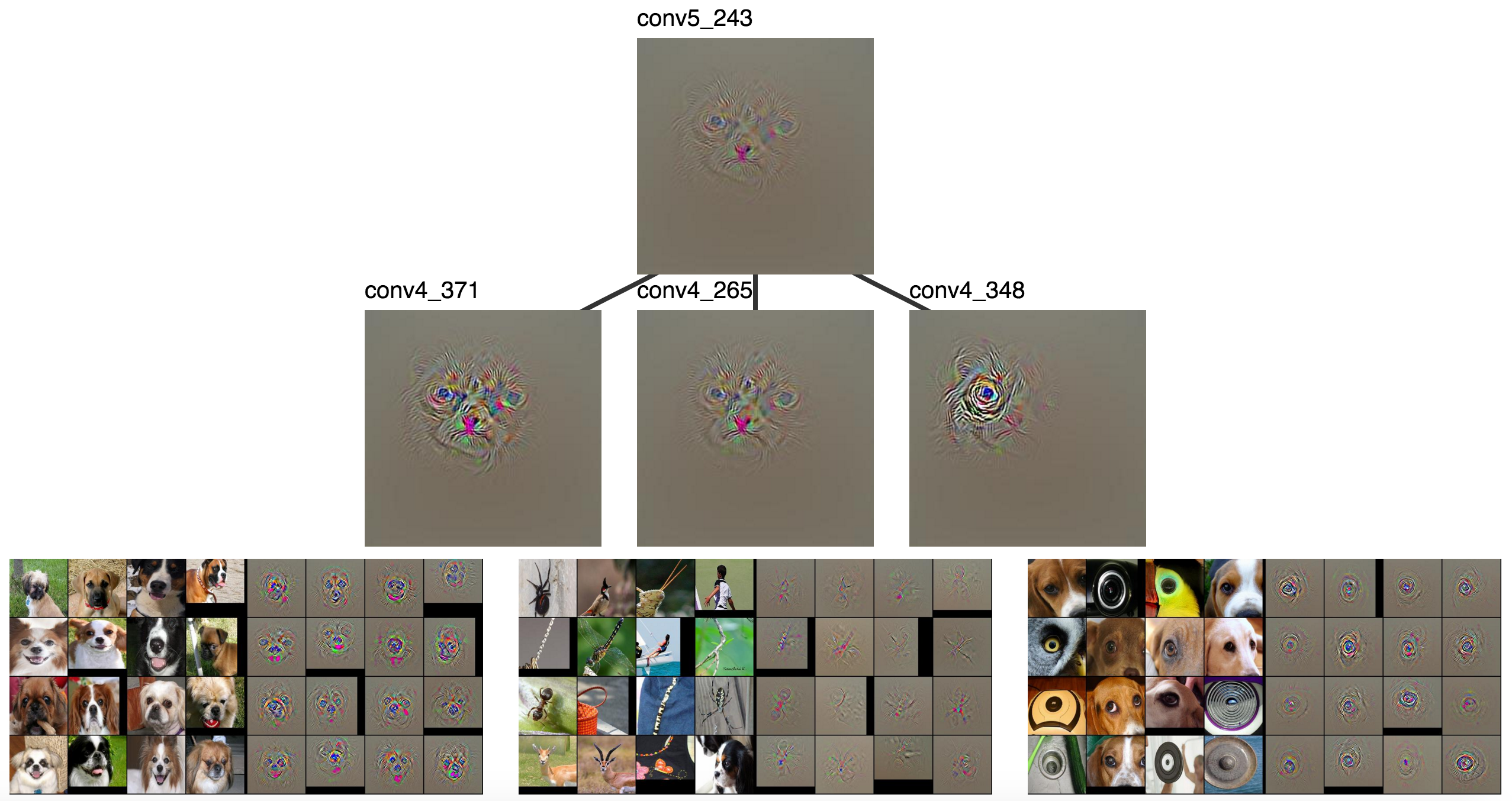
conv4_371, conv4_265, and conv4_348
There are lots face detectors (even in conv4!), some sort of pattern
that seems to find noses (conv4_265), and another eye detector.
I didn’t try to find the redundant face and eye detectors, they
just seem to occur quite frequently. There’s also a noticable difference in the amount
of complexity and context around the eyes and faces, with more complexity and
context in deeper layers.
dog faces + nose + eye + … = dog face
I’m still interested in faces, so let’s look at conv4_371.
We’ll throw out 2 neurons
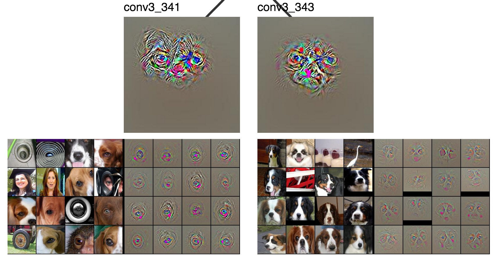
conv3_341 and conv3_343
and keep the rest.
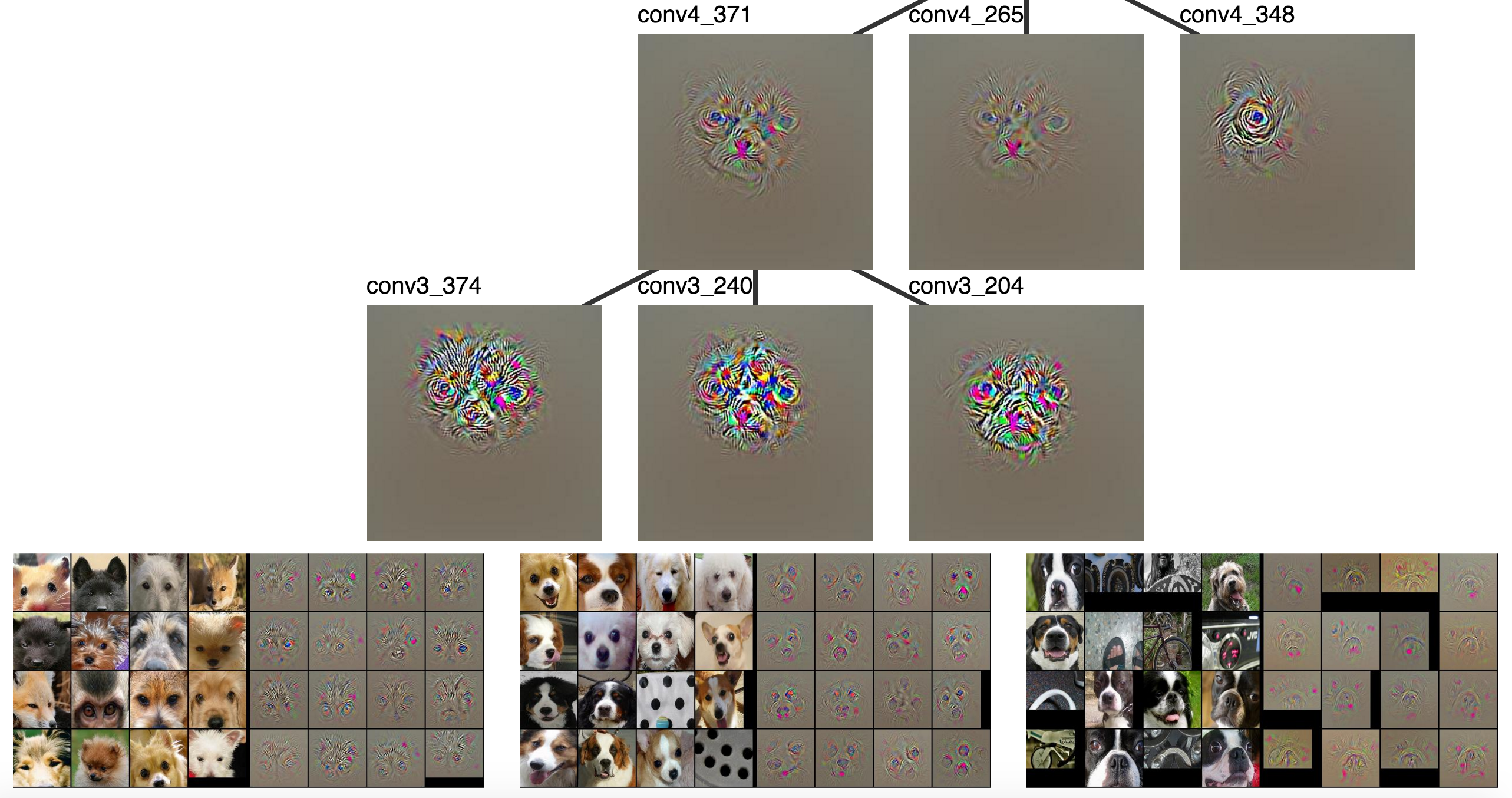
conv3_374, conv3_240, and conv3_204
We got rid of a simple eye detector and a vertical white line / face detectors and kept some more interesting features.
conv3_374 looks for fur and eyes together, conv3_240 looks for two eyes and a nose, and conv3_204
looks for a snout with a pink thing (tongue) underneath it.
face + eye +
conv3_374+conv3_240+conv3_204+ … = dog face
Clearly conv3_374, conv3_240, and conv3_204 are somewhat well defined parts,
but it’s hard to name them.
We’ll continue with conv3_240.
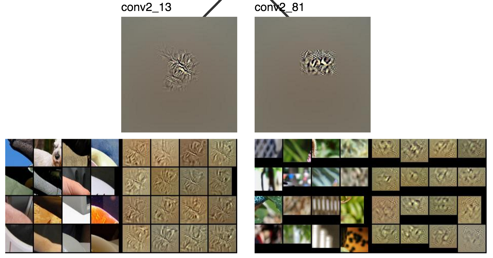
conv2_13 and conv2_81
The left neuron (conv2_13) sort of looks like it activated
for the cat’s cheek, but I can’t quite tell what the right one does.
These are clearly lower level than conv3, where there was still
a simple eye detector and a simple face detector.
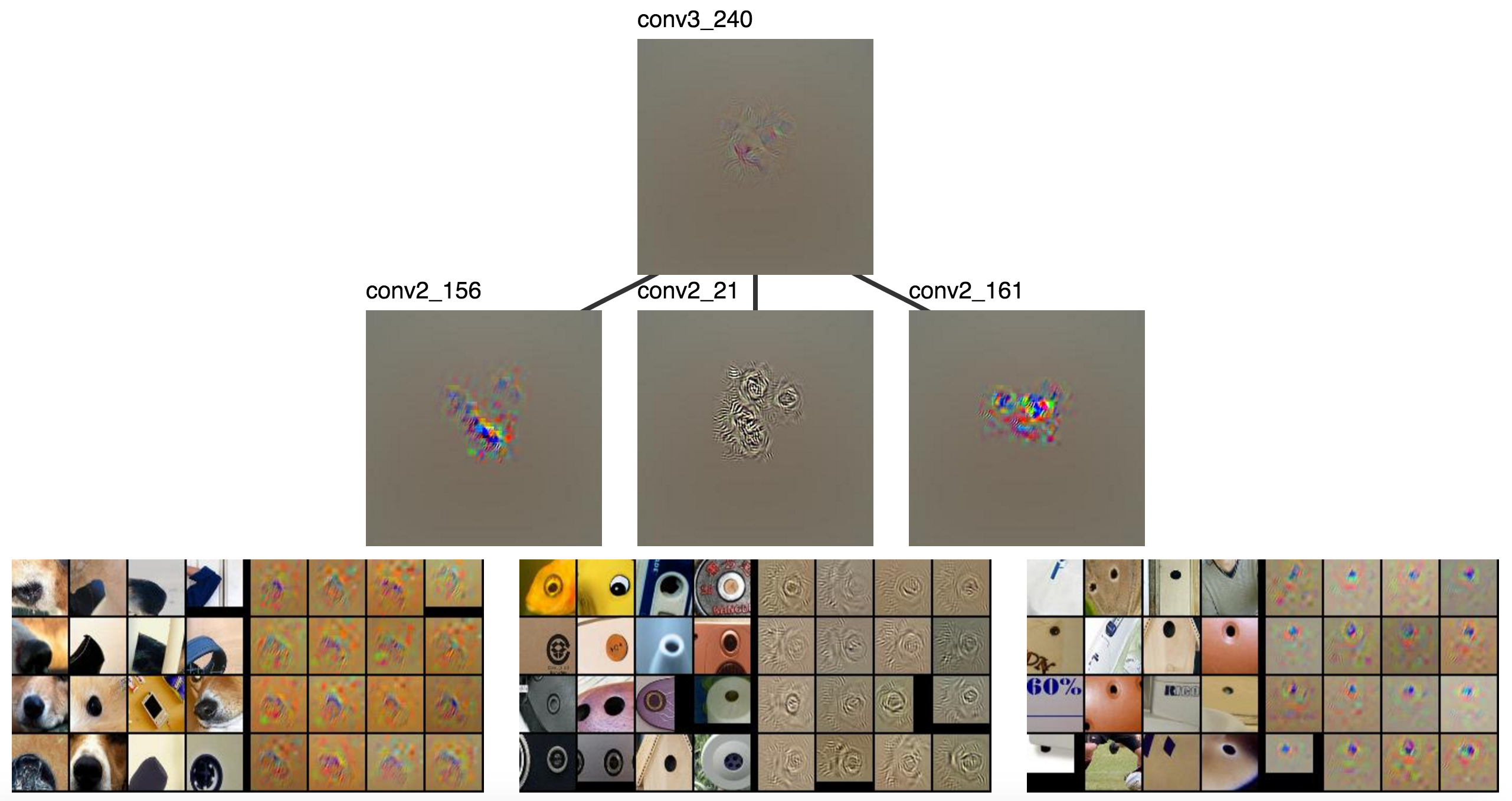
conv2_156, conv2_21, and conv2_161
I can see how conv2_161 and conv2_21 might be combined to create an eye detector
where the first looks for insides of eyes and the second looks for outlines. conv2_156
might also be used for noses, but it’s not a very strong connection.
dark black rectangular blob (nose) + circle outline (eye part 1) + small dot (eye part 2) + … = 2 eyes + nose
Finally, we visualize conv1, which looks for straightforward motifs
like the classic Gabor filters.
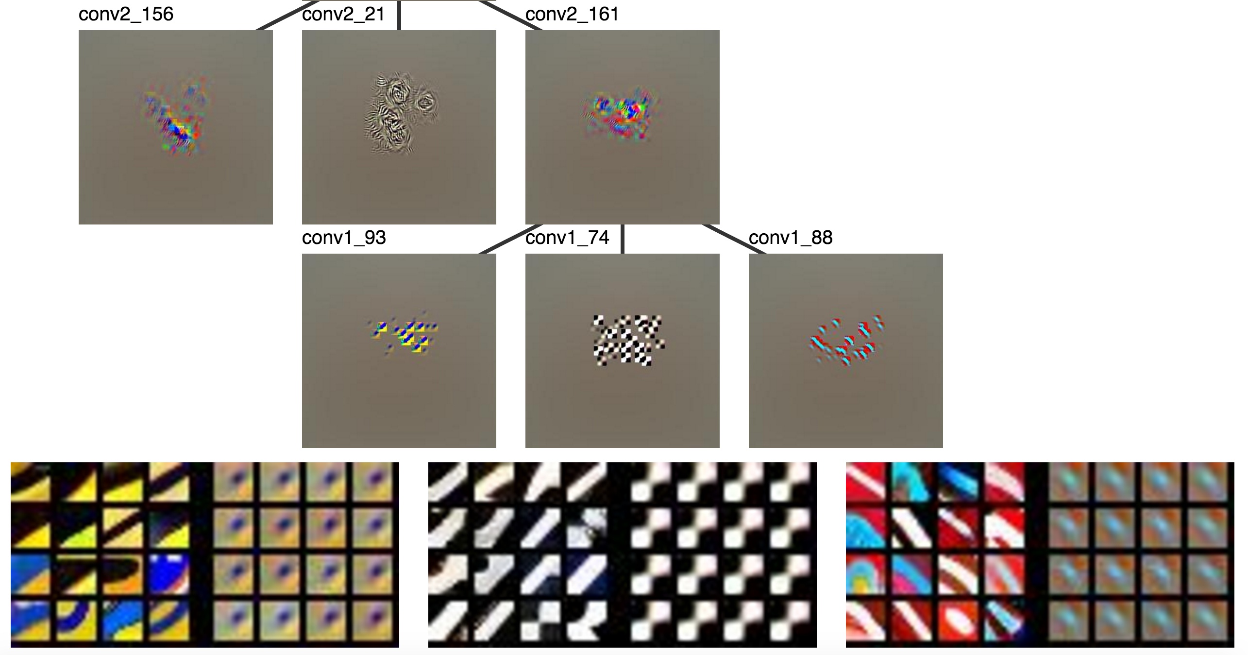
conv1_93, conv1_74, and conv1_88
circular blob + black and white grid + colored edge + … = small dot
The visualizations sort of answered why the CNN called the image a cat. The concepts represented by a neuron’s visualization and that of its parent typically fit together well. You can see how one is composed of the other. However, the visualizations, our capacity to understand them, or the network breaks down at some point.
Another interesting observation is the amount of redundancy between layers. For example, multiple layers seem to contain more than one face detector. It could be that the visualizations aren’t good enough to distinguish between features that really are different, that the network really learns redundant features, or that humans could do a better job at seeing the differences. Some of my recent work suggests the networks do learn significantly redundant features, so the models could be at fault.
Conclusion
In this post I explored how we understand ConvNets through visualization. We tend to focus on individual neurons, but not how they relate to other neurons. The latter part is essential because ConvNets are supposed work by learning to compose complex features from simpler ones. The second part of the blog proposed a way to combine existing visualizations in a way that relates units across layes in a neural network. These visualizations offer some insight into relations between features in adjacent layers, but this is only a small step toward a better understanding of ConvNets.
-
It looks like parallel coordinates, but it’s not really. The axes correspond layers of a CNN and the values on each axis correspond to individual neurons. Placing neurons on an axis implies an order (e.g., neuron 5 is greater than neuron 88), but no such ordering of neurons in the same layer exists. ↩
-
This tends to saturate visualizations, especially as they grow further from the root activation. I couldn’t find simple rule that consistently prevented saturating, but I found the saturated versions still work work well enough. Let me know if you come up with something. ↩